Kuramoto in Python

Dawid Laszuk published on March 02, 2017

7 min, 1229 words

Code for Kuramoto in Python is available here or from code subpage. Explanation on how to use it is on the bottom of this post.

Tiny introduction

Kuramoto^{[1, 2]} is probably one of the most popular and successful models for coupled oscillators. There is plenty of information about it, but in brief summary it models oscillators' phases to be dependent on scaled phase differences for all pairs of oscillator.

A while ago I have actually wrote on a specific method that I used to find optimal parameters for a Kuramoto model given some observation. (See Bayesian Dynamic Inference here.)

Mathematically speaking this model is defined by a set of coupled ordinary differential equations (ODEs). Given N oscillators, dynamics for each oscillator's phase $\phi_i$ is defined as $i\in N$ is defined by $\dot\phi_i = \omega_i + \sum_{j=0}^N k_{ij} \sin(\phi_i-\phi_j)$, where the summation is over all others oscillators. Note that one can leave coupling with itself, because in such case $\sin(\phi_i - \phi_i) = 0$, thus it doesn't input anything into the final solution.

Quick note that Kuramoto coupling model can be used to reference model with coupling function that can be represented as a sum of harmonic functions. For example, second order means that we are including both $k \sin(\Delta\phi)$ and $k^{(2)}\sin(2\Delta\phi)$. In general Kuramoto model of order $M$ would describe $\dot\phi_i = \omega_i + \sum_{m=0}^{M} \sum_{j=0}^N k_{ij}^{(m)} \sin(m (\phi_i-\phi_j))$.

Examples

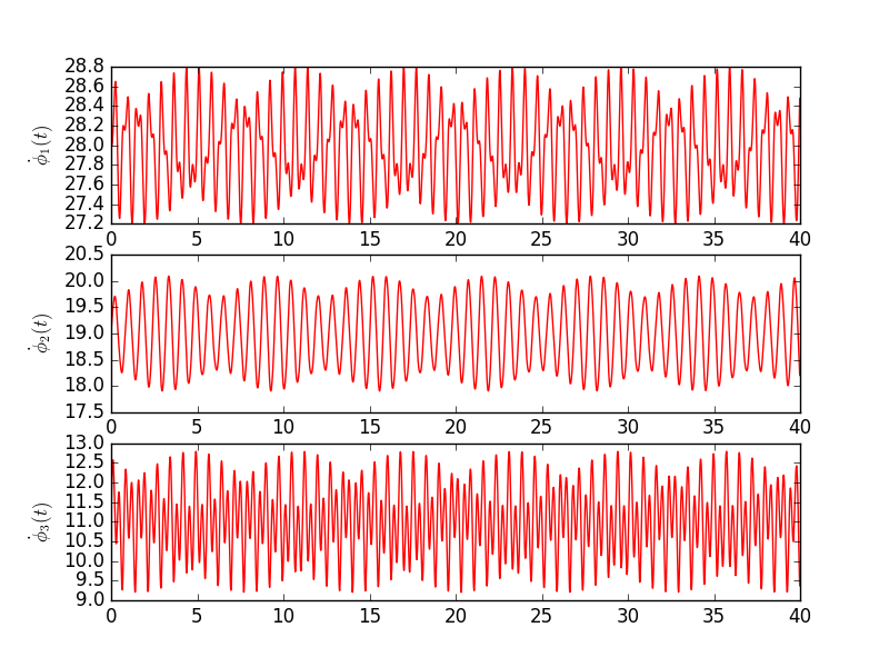
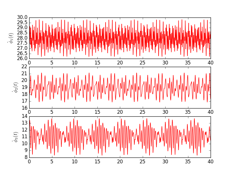
Below are two examples. Both use the same core values with the exception that for the second system the coupling function defined by two harmonic terms. This naturally changes dynamics, but it shouldn't change much average value, which is close to intrinsic frequency.

Exact values for the first experiment are presented in table below. Each row is a different oscillator with initial phase Φ₀ and intrinsic frequency Ω. The following columns denote coupling strength between respective pairs of oscillators.

	Φ₀	ω	k_.1	k_.2	k_.3
1	0	28		0.2	1.1
2	π	19	0.5		-0.7
3	0	11	0.3	0.9

Phase dynamics, i.e. time derivative of obtained phases, are presented in Fig. 1. One can see that all plots are centred on intrinsic frequency with some modulations.

Fig. 1. Phase dynamics, i.e. time derivative, in simple Kuramoto model.

Table below shows values used in the second simulation. Extra 3 columns denote scaling values used in second harmonic.

	Φ₀	ω	k⁽¹⁾_.1	k⁽¹⁾_.2	k⁽¹⁾_.3	k⁽²⁾_.1	k⁽²⁾_.2	k⁽²⁾_.3
1	0	28		0.2	1.1		-0.5	0.2
2	π	19	0.5		-0.7	-0.4		1.0
3	0	11	0.3	0.9		0.8	0.8

Again phase dynamics have been presented in a form of plot (Fig. 2). I think the difference is clear. Despite having similar mean values (approximately equal to intrinsic frequency), their modulations have change. Not only the frequency content of these modulations has changed, but also their amplitude.

kuramoto_dphi_2harmonic — Fig. 2. Phase dynamics, i.e. time derivative, in Kuramoto model with included second harmonic.

Using code

Except for downloading code from either github or code subpage, one is expected to have SciPy module. Kuramoto uses it to solve differential equations.

Script below shows an example of how one can use the Kuramoto module. When you run this, make sure that kuramoto.py is either in your path. Note also that most of the code is to just defining initial parameters and plotting the results. Actual execution of the module are two lines. Fig. 1 is the expected output.

import numpy as np
import pylab as plt
from kuramoto import Kuramoto

# Defining time array
t0, t1, dt = 0, 40, 0.01
T = np.arange(t0, t1, dt)

# Y0, W, K are initial phase, intrinsic freq and
# coupling K matrix respectively
Y0 = np.array([0, np.pi, 0])
W = np.array([28, 19, 11])

K1 = np.array([[  0, 0.2,  1.1],
               [0.5,   0, -0.7],
               [0.3, 0.9,    0]])

K2 = np.array([[   0, -0.5, 0.2],
               [-0.4,    0, 1.0],
               [ 0.8,  0.8,   0]])
K = np.dstack((K1, K2)).T

# Passing parameters as a dictionary
init_params = {'W':W, 'K':K, 'Y0':Y0}

# Running Kuramoto model
kuramoto = Kuramoto(init_params)
odePhi = kuramoto.solve(T)

# Computing phase dynamics
phaseDynamics = np.diff(odePhi)/dt

# Plotting response
nOsc = len(W)
for osc in range(nOsc):
    plt.subplot(nOsc, 1, 1+osc)
    plt.plot(T[:-1], phaseDynamics[osc])
    plt.ylabel("$\dot\phi_{%i}$" %(osc+1))
plt.show()

[1] Y. Kuramoto, "Chemical Oscillations, Waves, and Turbulence," 1984, doi: 10.1007/978-3-642-69689-3.

[2] Steven H. Strogatz, "From Kuramoto to Crawford: exploring the onset of synchronization in populations of coupled oscillators," 2000, doi: 10.1016/S0167-2789(00)00094-4.