Bayesian inference in Kuramoto model

For a while now, I've been involved in Kuramoto models and adjusting them to data. Recently I've stumbled upon using Bayesian inference on predicting parameters in time-evolving dynamics. Team from Physics Department at University of Lancaster has produced many papers, but to provide with some reference it might be worth to look at [1].

Technique refers to general phase $\phi$ dynamics in oscillator, i.e. $\dot\phi_i = \omega_i + f_i (\phi_i) + g_i (\phi_i, \phi_j) + \xi_i $, where $\omega_i, f_i(\phi_i)$ and $g_i(\phi_i, \phi_j)$ are intrinsic frequency, self coupling and coupling with other oscillators, respectively. Term $\xi_i$ refers to noise and although authors claim that it can be any type of noise calculations are performed for white Gaussian type. I don't really want to go much into details, because on first sight it might look complicated. Just to point out few steps that are necessary to introduce my examples:

1. Rewrite model in form of $\dot\phi_i = \sum_{k=-K}^{K} C_{k}^{(i)} P_{i,k} (\Phi) + \xi_i(t)$, where $c$ is parameters vector, $P$ provides significant terms (for example via Fourier decomposition) for our model and $\Phi$ is a vector of all oscillators' phases (at some moment).
2. Calculate diagonal values of Jacobian matrix, i.e. $\frac{\partial P_{i,k}}{\partial \phi_{i}}$.
3. Set a priori probabilities for parameters $C$ vector and its covariance $\Sigma$ (or concentration $\Xi = \Sigma^{-1}$).

Then the problem is reduced to finding maximum of minus log-likelihood function S. Authors also provide the exact formulas and algorithm, which find the extremum. Tutorial on applying their algorithm can be found in [2].

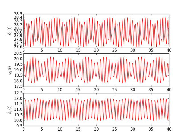
Based on MatLab code provided be the authors, and available on their webpage [3], I have written my own program in Python (code available in Code section or here ). As an experiment I have used simple Kuramoto model with sinusoidal coupling between phases $$\dot\phi_1 = 28 - 0.3 \sin( \phi_1 - \phi_2) - 0.1 \sin( \phi_1 - \phi_3 ) + 0.0 \sin( \phi_2 - \phi_3),$$ $$\dot\phi_2 = 19 + 0.3 \sin( \phi_1 - \phi_2) + 0.0 \sin( \phi_1 - \phi_3 ) - 0.9 \sin( \phi_2 - \phi_3),$$ $$\dot\phi_3 = 11 + 0.0 \sin( \phi_1 - \phi_2) + 0.1 \sin( \phi_1 - \phi_3 ) + 0.9 \sin( \phi_2 - \phi_3),$$ which means there are 12 parameters - three intrinsic frequencies ($\omega_i = {28, 19, 11}$) and 3x3 K matrix representing coupling between pairs of oscillators. To each oscillator small Gaussian noise was added (mean 0 and standard deviation 0.01). Signals were generated for $t \in [0, 40]$ with sampling step $dt = 0.001$. Furthermore, analysis was performed on 8 s segments with 2 s step. Figure 1 shows instantaneous frequencies ($\dot\phi_i$) for each oscillator. Figure 2 presents calculated parameters for each segment (thus time dependency). To be honest, I am quite surprised how good this technique works. I have performed more experiments, but to keep it short I am posting just one. There are some fluctuations in obtained values, but those changes are very small and most likely, in practical sense, negligible.

References

[1] A. Duggento, T. Stankovski, P. V. E. McClintock, and A. Stefanovska, “Dynamical Bayesian inference of time-evolving interactions: From a pair of coupled oscillators to networks of oscillators,” Phys. Rev. E - Stat. Nonlinear, Soft Matter Phys., vol. 86, no. 6, pp. 1–16, 2012.

[2] T. Stankovski, A. Duggento, P. V. E. McClintock, and A. Stefanovska, “A tutorial on time-evolving dynamical Bayesian inference,” Eur. Phys. J. Spec. Top., vol. 223, no. 13, pp. 2685–2703, 2014.

[3] Nonlinear Biomedical Physics, Lancaster University http://py-biomedical.lancaster.ac.uk/.