Particle Swarm Optimisation in Python

[Updated version available. See newest post.]

tl;dr: For Python PSO code head to codes subpage.

One might expect, that currently there is everything on the internet and it's only a matter of time to find something of an interest. At least that's what I expected. Unfortunately, sometimes finding the right thing and adjusting it to your own problem can take much more time that doing it yourself. This is a rule about which I often forget. And it happened again. I was suggested to try Particle Swarm Optimisation (PSO) for my problem. Since it has been some time since the introduction of that method, and since Python is a quite popular language, I expected that finding code to just do that wouldn't be a problem. True, it wasn't hard for few entries, but either software used some obsolete packages, or it was difficult to install it, or the instructions weren't clearly (to me) written. Thus, after about 2 days of trying to figure out everything and apply it to my problem, I simply gave up. That is, gave up searching and wrote my own code. In about 2 h.

What is Particle Swarm Optimisation (PSO)? Wikipedia gives quite comprehensive explanation, with a long list of references on this subject. However, in just few words: PSO is a metaheuristic, meaning that it does not require any a priori knowledge on gradient or on space. It is an optimisation method with many units (particles) looking independently for the best solution. Each particle updates its position (set of parameters) depending on its velocity vector, the best position it found during search and the best position discovered by any particle in swarm. Algorithm makes all particles go towards the best known solution, however, it does not guarantee that the solution will be globally optimal.

Algorithm depends on: initial positions $\vec{P}_0$, initial velocities $\vec{V}_0$, acceleration ratio $\omega$ and influence variable of the best global $\phi_g$ and the best local $\phi_l$ parameters. One also has to declare how many particles will be used and how many generations is the limit (or what is acceptable error of solution).

My program (shared in a Code section) can be executed in the following way:

pso = PSO( minProblem, bounds)
bestPos, bestFit = pso.optimize()

where minProblem is a function to be minimised (for an array of N parameters), and bounds is 2D (2 x N values) array of minimum and maximum boundary values. The bestPos is the best set of parameters and bestFit is smallest obtained value for the problem.

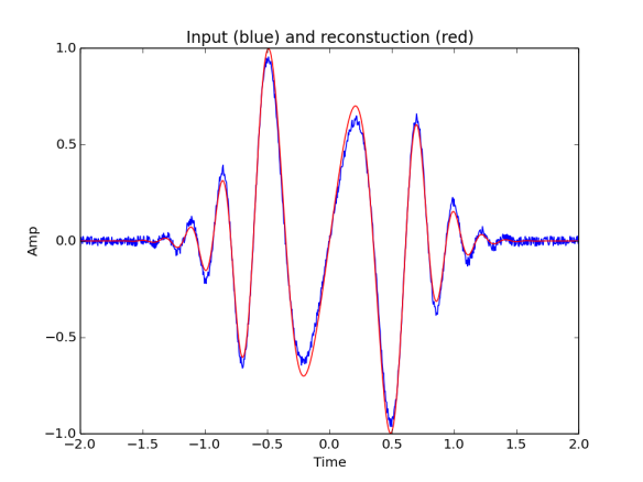
A small example provided with the code fits a curve to noisy data. Input signal was $S(t) = 4 t \cos( 4 \pi t^2) \exp(-3 t^2) + U(-0.025, 0.025)$, where $U(a,b)$ is a random noise from unitary [a, b] distribution. Fitted function is $F_{p}(t) = p_1 t \sin( p_2 \pi t^2 + p_3) \exp(- p_4 t^2)$, thus the expected values are P={4, 4, pi/2, 3}. See figure for fitted curve below. Obtained values are P = { 4.61487992 3.96829528 1.60951687 3.43047877} which are not far off. I am aware that my example is a bit to simple for such powerful search technique, but it is just a quick example.