EMD as dyadic filter bank
Soon after EMD was proposed researchers started analysing it and testing it for different sorts of applications. And obviously for papers, but it follows the other. One of the first discovered behaviours was acting as a dyadic filter bank on random data. This was shown in 2004 both on fractal Gaussian noise [1] and on white noise [2]. Those are very interesting papers and definitely worth reading.
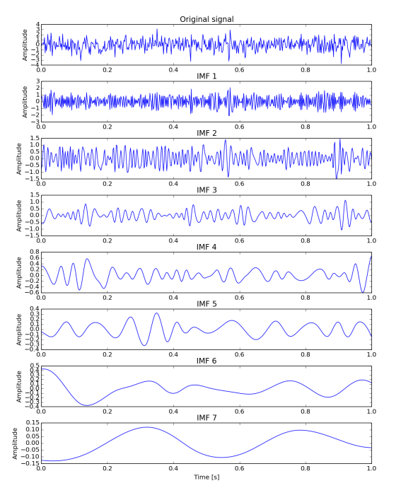
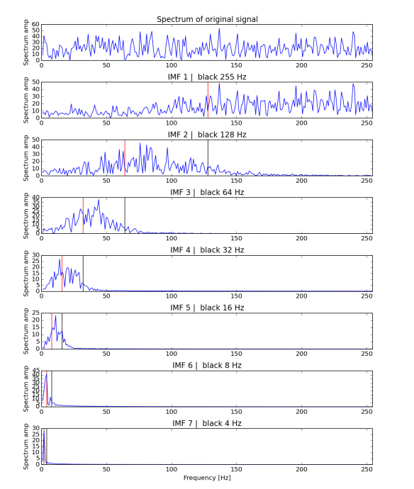
Quick example of such behaviour is presented in Figures 1 and 2. The first one shows input data - 256 data samples of normal random noise with 0 mean and variance 1 - and its EMD decomposition. Each row relates to different IMF. Figure 2 presents Fourier spectrum for signals in Figure 1, i.e. first row is spectrum for whole signal, second is for first IMF, third for second IMF and so on. Vertical lines relates middle (red) and end (black) of dyadic (powers of two) bands. Values of those lines are given as 256/n^2 and 256/(n+1)^2 respectively for black and red. Although they are not ideal they fit quite nicely and closely.
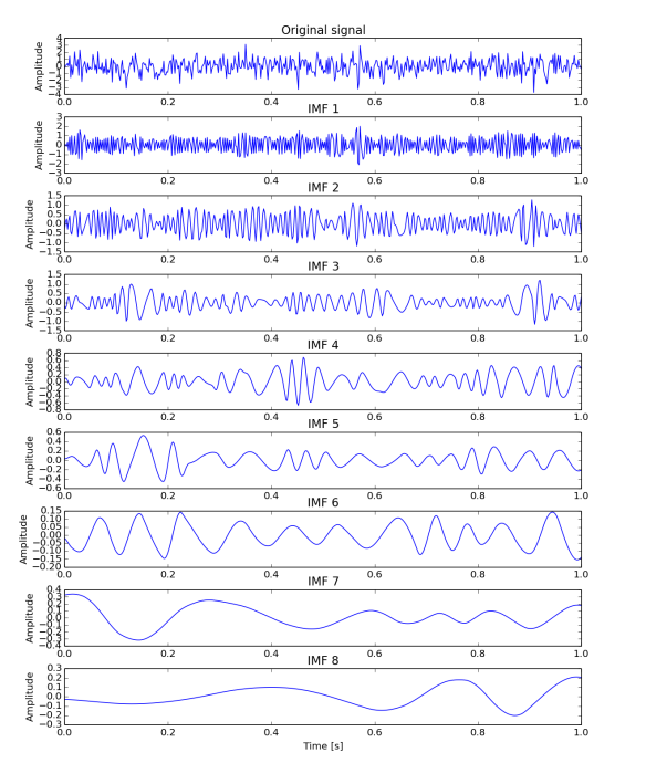
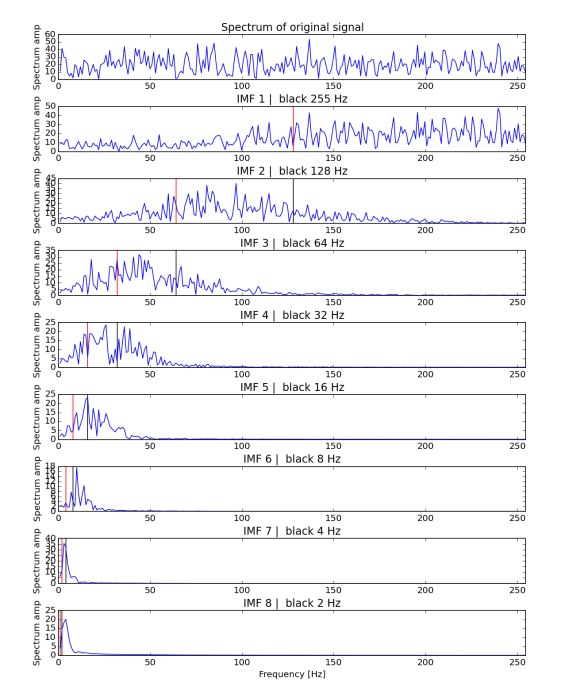
What is the reason for such behaviour? Actually it's not understood well. It has been show empirically that it exists, but as many EMD related features it lacks of mathematical explanation (again, [1] and [2] discuss this very nicely). Definitely it has to do with the type of input data (EMD on signal with 2 modes will replicate those modes, see previous post) and... spline types. Figures 3 and 4 shows exactly he same features as Figures 1 and 2, but where produced using Akima spline technique instead of Cubic natural splines. It can be seen that the vertical lines are not as close matching in Fig. 4 as they are in Fig. 2.
[caption id="attachment_204" align="aligncenter" width="584"]
 1) EMD decomposition of normal random data. First row is the input signal and the following relate to respective IMF. Plots are not in the same y scale.
[/caption]
[caption id="attachment_203" align="aligncenter" width="584"]
 2) Fourier spectrum made for original data and each IMF. Red and black vertical lines indicate respectively mean and end of filter bands. The exact values are powers of 2 - 256/(n+1)2 for red and 256/n2 for black, where n is the number of IMF. Plots are not in the same y scale.
[/caption]
[caption id="attachment_202" align="aligncenter" width="584"]
 3) EMD, using Akima's spline instead of natural cubic, performed on normal random data. First row is the input signal and the following relate to respective IMF. Plots are not in the same y scale.
[/caption]
[caption id="attachment_201" align="aligncenter" width="584"]
 4) Fourier spectrum made for original data and each IMF from Fig. 3 (using Akima's splines). Red and black vertical lines indicate respectively mean and end of filter bands. The exact values are powers of 2 - 256/(n+1)^2 for red and 256/n^2 for black, where n is the number of IMF. Plots are not in the same y scale.
[/caption]
[1] P. Flandrin, G. Rilling, and P. Goncalves, “Empirical Mode Decomposition as a Filter Bank,” IEEE Signal Process. Lett., vol. 11, no. 2, pp. 112–114, Feb. 2004. [2] Z. Wu and N. E. Huang, “A study of the characteristics of white noise using the empirical mode decomposition method,” Proc. R. Soc. A Math. Phys. Eng. Sci., vol. 460, no. 2046, pp. 1597–1611, Jun. 2004.