Ensemble empirical mode decomposition (EEMD)
As mentioned in previous posts, one of the main drawbacks of EMD is its poor stability. This means that slight changes to input signal will cause changes in the output. Sometimes small, sometimes big, but almost always some changes. Ensemble empirical mode decomposition (EEMD) [1] is based on the assumption that small perturbations to input signal will also perturb slightly results around the true output. In fairness, we don't know whether the data we are using are noise free (almost never they are) and this contamination itself affects the output.
How does EEMD work? It creates a large set (an ensemble) of EMD boxes. Let's assume there are N of those boxes, but typically $N \geq 100$. Each of them process data s(t), but with artificially injected noise n(t). The true result is a grand average over all sets for each component, i.e. $c_j(t) = \frac{1}{N} \sum_{i=0}^{N} EMD_j \left[ s(t) + n_i(t) \right]$, meaning that component j is a grand average of all j components for each contaminated i data out of N sets. This should work because of the noises' zero mean property. Originally it was suggested to use random white noise distribution with a finite amplitude of 0.2 data's standard deviation. It was also mentioned that type of distribution and amplitude parameter are not optimal for all choices and one should adjust them for one's own purpose. Another assumption is that all components have two parts: one related to true results and a pure noise, which again, because of mean property, should on average cancel each other out.
The original article, like all Huang's, ale really well written and gives throughout view with pros and cons of the method. Although it is still very much empirical it has been applied, with success, to many problems (multidimentional decomposition [2] or artifact removal from biosignals [3]). Moreover, because of its straight forward parallel computing nature, there are many attempts to create GPU-sutiable computing algorithms [4, 5].
As a example I have generated a signal s(t) composed of 3 sine waves: $s(t) = -(3 \cos(2\pi \cdot 4t) + 4 \sin(2\pi \cdot 13t) + \sin(2\pi \cdot 21t))$. This signal is displayed in Figure 1. Fairly to say it is not complicated function.

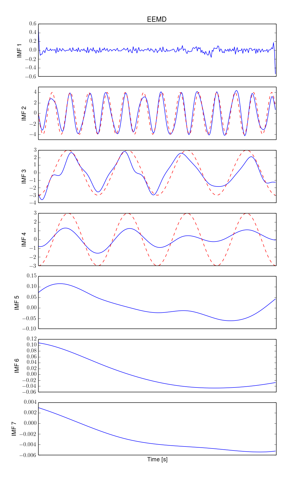
Signal s(t) has been processed with both EMD and EEMD which results are presented on Figures 2 and 3 respectively. Additionally, on those figures, expected sine waves (the ones with similar frequencies) have been added coloured with red dashed lines. These examples are just to present possible outcomes of the methods rather than promote any of them, thus results are not the most "outstanding". One can see that both methods have returned 2 slower components and completely omitted the fastest 21 Hz component.
There are few things here worth noting about EEMD. First of all, EEMD's first component is always related to generated noise. Again, this is empirically "proven", but it makes sense. Since we are using noise, i.e. fastest changing signal, and EMD returns IMFs from the highest frequency first, thus it shouldn't be surprise to obtain noise related component in each performed EMD of ensemble. Secondly, the first component should usually be close to zero due to being sum of zero mean random numbers. Personally, I haven't read anyone advocating this to be one of EEMD sensibility test, but since we are posing noise cancellation and we know that the first component is mostly related to them, then in my opinion, it should. Thirdly, returned components are not necessarily IMFs in original definition, i.e. their local mean is not always 0. It is simple result of adding (in grand average) two or more signals that are not phase synchronised and probably have different "frequencies". For different injected noises EMD can produce different number of IMFs, which sometimes forces addition of components that most likely are not related to the same feature.

As a bonus, I have made EEMD of null signal (no signal) using exactly the same noise components as in presented example. Figure 4. presents the output. Unsurprisingly, the components are still not IMFs, but they preserve the order of average frequency, i.e. the average frequency decreases with increase of the component's order number.

References
[1] Z. Wu and N. E. Huang, “Ensemble Empirical Mode Decomposition: a Noise-assisted Data Analysis Method,” Adv. Adapt. Data Anal., vol. 1, no. 1, pp. 1–41, Jan. 2009.
[2] Z. Wu, N. E. Huang, and X. Chen, “The multi-dimensional ensemble empirical mode decomposition method,” Adv. Adapt. Data Anal., vol. 1, no. 03, pp. 339–372, 2009.
[3] K. T. Sweeney, S. F. McLoone, and T. E. Ward, “The use of ensemble empirical mode decomposition with canonical correlation analysis as a novel artifact removal technique.,” IEEE Trans. Biomed. Eng., vol. 60, no. 1, pp. 97–105, Jan. 2013.
[4] L.-W. Chang, M.-T. Lo, N. Anssari, K. Hsu, N. E. Huang, and W. W. Hwu, “Parallel implementation of Multi-dimensional Ensemble Empirical Mode Decomposition,” in 2011 IEEE International Conference on Acoustics, Speech and Signal Processing (ICASSP), 2011, pp. 1621–1624.
[5] D. Chen, D. Li, M. Xiong, H. Bao, and X. Li, “GPGPU-aided ensemble empirical-mode decomposition for EEG analysis during anesthesia.,” IEEE Trans. Inf. Technol. Biomed., vol. 14, no. 6, pp. 1417–27, Nov. 2010.